Employee Attrition Analysis

Background

Canterra, a company of over 4000, has requested an in-depth analysis of their rate of attrition. The company experiences a large exodus of about 15% of its employees each year, in which the replacement process of these employees requires valuable time and resources. Employees may leave for a multitude of reasons, such as the termination of their employment or their own personal decision to leave. 

Canterra believes that this level of attrition has a number of negative consequences for the company. Management has listed three consequences: First, having a poor rate of attrition can cause projects to become delayed due to the difficulty in meeting timelines as a result of the decrease in employees. This affects the image and reputation of the company. Second, resources are spent on maintaining a large recruiting department; something that Canterra would like to see change. Third, new employees have to be trained on their new positions, which takes time, especially if the new employee came to Canterra with limited or no experience. These variables, and more, will be reviewed as part of this analysis.

Executive Summary

This analysis is a deep dive of every variable in the dataset provided by Canterra’s management team. While the initial analysis, which used logistic regression, only took into account the variables that management at Canterra believed were impacting attrition, our deeper analysis, which utilized decision trees, bagging and random forest took into account all variables as our team believed that we could provide further insight into why Canterra has been experiencing a 15% exodus. We found that age, income, years at Canterra, distance from home, and the number of companies an employee has worked at were the most powerful predictors of attrition. This will be discussed in detail in the following assessment. 

Ultimately, we believe that incentives, such as performance bonuses, and higher salaries for entry level positions would entice younger employees to remain at Canterra. We hypothesize that younger employees are more prone to leave given the significance of the age and income variables. Additionally, we feel as though the freedom to switch teams if an employee does not like their manager is important. Intuitively, the longer an employee remains with their manager, the more they enjoy working for that manager. The more favorable an employee’s experience with their manager, the less likely they are to leave the company in search for a new manager. 

Logistic Regression Methods and Diagnostics 

The logistic regression model was created in its entirety in R Studio using a multitude of packages that include, but are not limited to Caret, ROSE, Car, ROCR, etc. The model was built with a dataset provided by Canterra that covered a number of factors including age, employee ID, income, job level, marital status, etc. Our variables of interest, due to the request and assumptions of Canterra’s management team, were Job Satisfaction, Total Working Years, Years at the Company, Age, Gender and Education. Other variables were omitted. 

To start, the Employee Data dataset was loaded to R with accompanying packages needed for logistic regression and diagnostics. There were a number of variables that were read into R as characters that had to be converted to numeric values. Next, our Y variable, Attrition, was converted to a numeric; 1 indicating that the employee left the company and 0 indicating that the employee remained. The same conversion was done to our independent variable, Gender, where 1 indicated Male and 0 indicated Female. 

Next, the Employee Data dataset was partitioned randomly to reflect a 70% - 30% split between training and test data. We then evaluated the dataset for missing, NA, values, of which there were quite a few. In order to account for the missing data, the median value of each variable was taken and replaced with the missing observations. Downsampling was then performed to account for the imbalance between the minority and majority classes. As Canterra noted, around 15% of the company left. Intuitively, there is bound to be an imbalance in the Attrition variable of the dataset given that the majority of employees stay with the company. 

The first iteration of the logistic regression model was created with the downsampled data and the variables of interest. With the results of the first model iteration, we then checked for multicollinearity, of which there was none. Next, we used a stepwise regression approach to narrow down to the most significant variables. The stepwise regression model determined that Age, Years at the Company, Total Working Years and Job Satisfaction were the most significant variables affecting Attrition given that their p-values were below 0.05, denoting significance. 

Next, the coefficients of the stepwise model were examined. As can be seen in Appendix A: Odds Ratio of Stepwise Model, an increase in any of the independent variables results in a decrease in the odds of attrition, which we know given that all variables are less than 1. Interpretation of these results will be explained in the overview of attrition. Additionally, it should be noted that deviance decreased from 2721.4 to 2577.1. 

As can be seen in Appendix B: Performance and Accuracy Using Confusion Matrix, when using a sensitivity threshold of 0.5, the accuracy of our predicted values is high, at 84% with a 95% Confidence Interval of 81.7% at the lower limit and 85.7% at the upper limit, however, the data is very imbalanced. To account for the imbalance in the data, specifically the minority class, synthetic data was to be created to even out the classes. In other words, our goal was to increase the minority share of the Attrition variable (those who have left the company) by creating synthetic data by using oversampling. 

To account for the imbalance in our attrition variable, specifically the minority class, synthetic data was created to even out the classes using the ROSE package in R. Appendix C: Oversampling Results displays the accuracy of the oversampled data, which decreased from 84% to 67%, with a 95% Confidence Interval of 64.2% at the lower and 69.4% at the upper limit. 

According to the results of the receiver operating characteristic (ROC) curve and the area under the curve (AUC), the synthetic data provides the best model. As can be seen in Appendix D: ROC Curve and Appendix E: Oversampling ROC Curve, the AUC is .5 and .735 respectively. In other words, there is a 73.5% likelihood that the model using synthetic data will be able to distinguish between those who will leave Canterra and those who will remain. 

Decision Tree Methods and Diagnostics 

As an alternative to the logistic regression, we considered the rule-based decision tree. Based on our decision tree, the most important variables are Total Working Years, Years with Current Manager, Age, and Marital Status. If following this model, these would be the variables that management should address immediately. Somewhat important variables include Years at Company and Environmental Satisfaction. Less important variables include Business Travel, Number of Companies worked, Job Satisfaction and Training Times. Variables that were not considered are Distance from Home, Education, Gender, Job Level, and Income. 

Interpretation of Tree

If there are any “Yes” responses to our questions, such as whether an employee is married, then one would move down the left side of the tree split, while “No” responses would move down the right side of the tree split. A blue node indicated by “1” indicates likelihood of attrition and a green node of “0” indicates likelihood of retention. Our threshold is set at 0.50. If there is over a 50% chance, then the model predicts it as attrition.

Our decision tree indicates that we first consider whether or not the employee is married. This node makes up 100% of our employees. If employees are not married, we move down the right side to learn that 40% of all employees are single. These single employees have a 33% chance of staying at the company and 67% of leaving the company. Next, we consider whether they have been with their current manager for over 3.33 years. If they have not, we move down the right side to learn that 23% of all employees fall within this category. They have a retention rate of 24% and an attrition rate of 76%. Because the attrition rate is over 50%, the final node is blue and contains the number “1” - indicating the likelihood for attrition. On the opposite side of this tree, employees who are married or divorced (60% of all employees) and have worked for over 9.4 years (30% of all employees), have a 70% retention rate.

  Lastly, our decision tree model has a lower accuracy rate (0.59) and sensitivity rate (0.4976) compared to our baseline oversampled logistic regression model (Appendix F). The area under the curve (AUC) is 0.59, indicating that 59% of the time, the model can determine a true positive from a false positive case of attrition (Appendix J).

Methods: Decision Tree

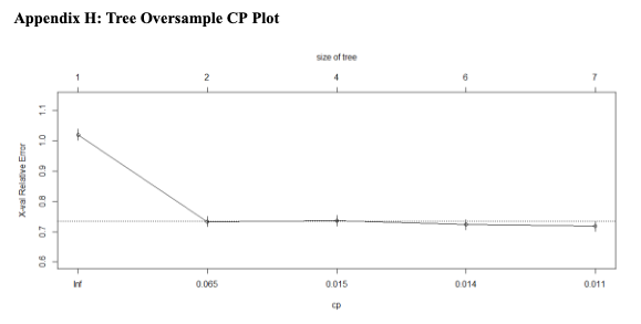
Continuing from the cleaned and split training and testing data, with the same seed, we oversampled the data through the ROSE package to have consistent data for comparison to our baseline logistic regression model. Oversampling provided a smaller set of trees with lower cross validation errors (default is 10-times cross validation) than compared to that without oversampling. While using the ROSE package, we also used a seed to ensure that the oversampling is reproducible. Next, using the RPARTS package, we created the categorical logistic regression decision tree and reviewed the CP table and plots (Appendix G & H). We considered whether or not to prune the decision tree. We did not prune the decision tree because the N-Split with the lowest CP was set at 6 splits (Appendix G). Pruning to a smaller tree may increase the predictive accuracy; but, it would offer less variables for an explanatory analysis.

Afterwards, we considered the variable importance of the decision tree to determine which variables needed to be addressed immediately (Appendix I). This is important because the variable with the highest importance is not necessarily the first variable to split in the decision tree. As an example, in our decision tree Marital Status was the first split; however, it ranked as the fourth in importance. Finally, for metrics, we passed the test data set into the model to create a confusion matrix for the oversample decision tree (Appendix F) and AUC plot (Appendix J).

Bagging Diagnostics and Methods

Single tree models can suffer from high variances. Pruning the tree helps reduce this but there are alternative methods that are better for prediction and for making a better model. Bagging (Bootstrap Aggregating) helps us combine and average multiple models, thus helping us to reduce variability of any one tree along with overfitting to improve our predictive performance. 

We used two methods to perform bagging and both had a similar RMSE. In performing bagging with Caret, we did a 10-fold cross-validated model. The cross-validated model of bagging using caret gives us a more robust understanding of the true expected test error than the OOB error. Our model had an RMSE of .322, showing that it could predict the data relatively accurately.

Our bagging model was able to predict attrition 85% of the time and retention 87%. The accuracy of this model was fairly accurate at nearly 87%. In assessing the variables, 16 of them, many contributed, but the most important ones that had a significant impact on our model were Income, Age, Distance from Home, Job Satisfaction, and Total Working Years. Variable importance for regression trees was assessed by taking the total amount SSE decreased by splits over a certain predictor and then averaged over all “m” trees. Then, the predictors with the largest impact on SSE were considered most important. This value of importance is simply the relative mean decrease in SSE when compared to the most important variable (0-100 scale). In essence in recognizing this and utilizing the bagging model, this highlights that management's focus should be on these top 5 variables as a means of improving attrition when considering bagging as the model of choice. – A thorough discussion of the methods can be found starting in Appendix H. 

Random Forest Diagnostics and Methods

A decision tree is a simple model to interpret; however, it mainly focuses on optimizing the node split rather than considering how it can affect the entire tree. Therefore, we considered using a Random Forest model, which would provide a more accurate model for the entire forest. Based on our model, shown above and in Appendix Q, the most critical variables are Income, Age, Total Working Years, Distance from Home, and Years at the Company. Therefore, we highly encourage management to promptly address these variables. As a note, variables contributing to a lower rate include Business Travel, Gender, and Standard Hours. 

Interpretation of the Model

Despite having focused on a smaller group of variables during our initial logistic regression model, within our random forest model, we decided to incorporate all the variables provided to us by Canterra to find which had high predictive power. A Random Forest model is best implemented to find higher accuracy and reliability. Therefore, our model underwent multiple cleaning and refining to come to our final model. However, as shown in Appendix M, our initial model produced a “true negative” (0) of 2,584 and a “true positive” (1) of 427, and an Out of Bag error of 2.46%. Therefore, from our observation, we can predict that 2,584 employees will stay at the company and 427 employees will leave. 

Additionally, from the given low OOB percentage, we can assume that a small number of variables should be tested simultaneously to ensure a small amount of error. As we refined our model, we increased the number of trees by 1,500 and tested six variables tried at each split. It resulted in a lower OOB and an increase in “true positive” and “true negative” numbers. As shown in Appendix R, OOB had decreased from 2.46% to 2.36%, while “true positives” increased to 2,580 and “true negatives” increased to 434. Thus, we conclude that the optimal test value at each split was six variables. In conclusion, Canterra’s management should focus on testing six variables to find the reason for employee attrition instead of 10+ variables, which can lead to a higher level of OOB error.

Furthermore, as shown in Appendix O, our random forest variable model has an extremely high accuracy rate of 96%, a sensitivity rate of 99%, and a specificity rate of 83% compared to our logistic regression model (Appendix F). While also having an extremely high confidence interval of 95.3% and 97.4%. This suggests that we could accurately predict 83% of the “0” and 99% of the “1”, allowing us to conclude that this is an excellent model. Comparatively, the area under the curve is 97%, as shown in Appendix P. Thus, there is a 97% chance that the model can correctly distinguish between a positive and a negative class. 

Lastly, we plotted each variable to test the predictive power of each. As shown in Appendix Q, we can conclude that income has the highest predictive power of over 100 and is the most significant factor for employee attrition. In addition, we can also see that age (100) and total working years (82) also have high predictive power. On the other hand, business travel, gender, and standard hours had the lowest predictive power. 

Methods: Random Forest

Continuing from the previous cleaned and split training and testing data with the same set seed, we oversampled the data through the randomForest package and also ensured that we used the same seed for the reproducibility of our data. Our result was 2,584 zeros (retention) and 427 ones (attrition), and an OOB error rate of 2.46%, as seen in Appendix M.

Next, as seen in Appendix N, we plotted our result data, including our out-of-bag error, to refine the accuracy of our random forest model. The first step we tested was to define the optimal number of variables tried at each split from 1 variable to 10 to find the most accurate out-of-bag error. As seen in Appendix R, within our testing, we found that six variables tried at each split were optimal and returned an OOB estimate of an error rate of 2.36%. 

Finally, we used our refined random forest to predict our test data. This resulted in a high level of accuracy, sensitivity, and specificity. As shown in Appendix Q, we plotted the above data to show importance based on each variable. The closer the variable is to 100 on the given plot, the greater the chance of it impacting the level of attrition. 

Overview of Attrition

In conclusion, out of the various models that our team ran, we ultimately decided that our Random Forest model was the best predictor of attrition. While decision trees are more easily comprehensible and while our decision tree model gave us a better measure of predictability, we suggest the Random Forest model and results given the higher degree of accuracy and reliability. 

If the leadership team prefers to review a model that can be quickly understood and implemented, you can consider using the decision tree with the caveat that its accuracy hovers around fifty percent. The logistic regression also provides information on the odds of a person leaving the company, and with slightly higher accuracy than the decision tree. This might also be an option, though it may not appeal as much to stakeholders who prefer a visual representation.

Below is a comparison of metrics from the four models that inform our final model. Across the four models, there were multiple recurring top variables, with the variables Age and Total Working Years consistently appearing in each model.

Recommendations

Our recommendations are based on the most powerful predictors of attrition, which, according to our model, are income, age, distance from home, years at Canterra, and the number of companies that an employee has worked at. Primarily, our results suggest that younger employees are prone to switching companies far more often than employees who have been with Canterra for many years. We recommend that Canterra offers competitive starting salaries along with incentives for good performance, such as a performance bonus. Younger employees will be enticed to remain at Canterra for longer given the guarantee that the performance bonuses will only increase with seniority. Additionally, we have found that longer an employee remains with their manager, the more likely they are to remain at the company. We recommend that employees have the freedom to switch teams if they are not satisfied with their manager. Canterra may also want to give young entry level employees the opportunity to work with multiple teams and remain with whichever manager they feel they are most comfortable and productive with. The more satisfied an employee is with their manager, the more likely they are to remain at Canterra. 

Appendices